File:Butterworth response.png
Original file (1,240 × 880 pixels, file size: 86 KB, MIME type: image/png)
Captions
Captions
Summary[edit]
| Description |
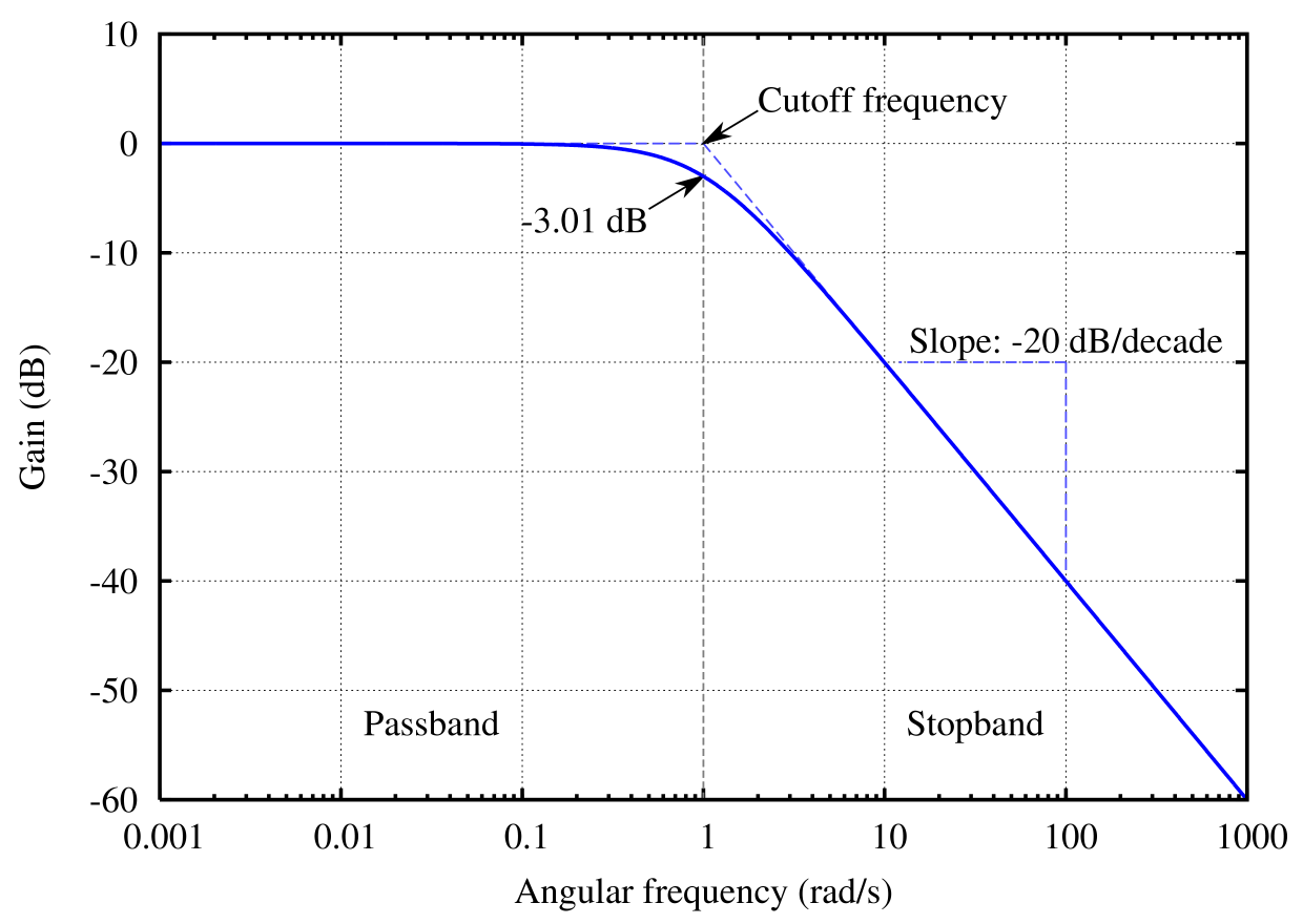
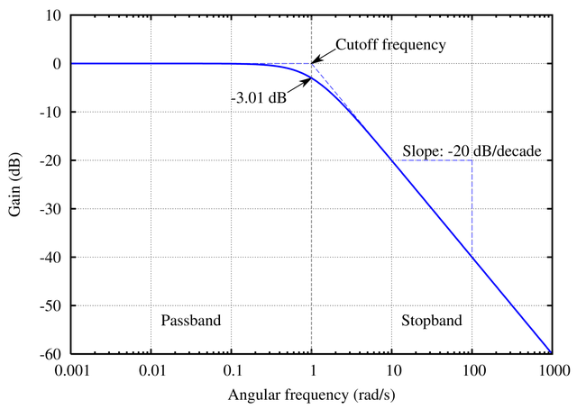
English: The frequency response of a Butterworth filter with logarithmic axes (Bode plot) and various labels. Cutoff frequency is normalized to 1 rad/s. Gain is normalized to 0 dB in the passband.
Many orders on one plot: File:Butterworth orders.png. Version with no text available at File:Butterworth plain.png, though you should probably just modify the source code and regenerate it in your own language. See Wikipedia graph-making tips. This plot was created with Gnuplot. Generated in gnuplot with the script below (save as butterworth.plt and then open in gnuplot). Then I opened the butterworth.ps file in a text editor to edit the line colors and linestyles, as per this description. This avoids needing to open in proprietary software, and really isn't that difficult (especially if you don't know the commands in the proprietary software either). ;-) Identify the lines easily by their color (the arrow is currently magenta and I want it to be black. Ah, there is the entry with 1 0 1, red + blue = magenta) or by using the gnuplot linestyle−1. (For instance, gnuplot's linestyle 3 corresponds to the ps file's /LT2.) Then you can edit the colors and dashes by hand. I changed the original: /LT0 { PL [] 1 0 0 DL } def
/LT1 { PL [4 dl 2 dl] 0 1 0 DL } def
/LT2 { PL [2 dl 3 dl] 0 0 1 DL } def
/LT3 { PL [1 dl 1.5 dl] 1 0 1 DL } def
into this: /LT0 { PL [] 0 0 1 DL } def
/LT1 { PL [4 dl 2 dl] 0.5 0.5 0.5 DL } def
/LT2 { PL [6 dl 3 dl] 0.3 0.3 1 DL } def
/LT3 { PL [] 0 0 0 DL } def
/LT4–/LT8 I left unchanged. (I don't know what they're used for anyway.) /LTw, /LTb, and /LTa are for the grid lines and such.To convert the PostScript file to PNG:
|
| Date | 26 June 2005 (upload date) |
| Source | Own work |
| Author | Omegatron |
| Other versions |
|
| gnuplot source | click to expand
set samples 2001
set terminal postscript enhanced landscape color lw 2 "Times-Roman" 20
set output "butterworth.ps"

# Butterworth amplitude response and decibel calculation.  n is the order, which is just 1 in this image.
G(w,n) = 1 / (sqrt(1 + w**(2*n)))
dB(x) = 20 * log10(abs(x))

# Gridlines
set grid

# Set x axis to logarithmic scale
set logscale x 10

# Set range of x and y axes
set xrange [0.001:1000]
set yrange [-60:10]

# Create x-axis tic marks once per decade (every multiple of 10)
set xtics 10

# Use 10 x-axis minor divisions per major division
set mxtics 10

# Axis labels
set xlabel "Angular frequency (rad/s)"
set ylabel "Gain (dB)"

# No need for a key
set nokey #0.1,-25

# Frequency response's line plotting style
set style line 1 lt 1 lw 2

# Draw a separator between passband and stopband and label them
set style line 2 lt 2 lw 1
set style arrow 2 nohead ls 2
set arrow 3 from 1,-60 to 1,10 as 2

# Label coordinates are relative to the graph window, not to the function, centered at the 1/4 and 3/4 width points
set label 1 "Passband" at graph 0.25, graph 0.1 c
set label 2 "Stopband" at graph 0.75, graph 0.1 c

# Asymptote lines and slope lines are the same "arrow" style
set style line 3 lt 3 lw 1
set style arrow 3 nohead ls 3

# Draw asymptote lines
set arrow 1 from 1,0 to 1000,-60 as 3
set arrow 2 from .001,0 to 1,0 as 3

# -3 dB arrow style and arrow
set style line 4 lt 4 lw 1
set style arrow 4 head filled size screen 0.02,15,45 ls 4
set arrow 4 from 2,3 to 1,0 as 4

# "Cutoff frequency" label uses same coordinates as the function
set label 3 "Cutoff frequency" at 2,4 l

# "-3 dB" label
set arrow 5 from 0.5,-6 to 1,-3 as 4
set label 4 "-3.01 dB" at 0.5,-7 r

# Draw slope lines and label
set arrow 6 from 100,-20 to 12,-20 as 3
set arrow 7 from 100,-20 to 100,-39 as 3
set label 5 "Slope: -20 dB/decade" at 100,-18 c

# Plot the filter response
plot \
     dB(G(x,1)) ls 1  title "1st-order response"
|


|
File:Butterworth response.svg is a vector version of this file. It should be used in place of this PNG file when not inferior.
File:Butterworth response.png → File:Butterworth response.svg
For more information, see Help:SVG. |
 |
Licensing[edit]
- You are free:
- to share – to copy, distribute and transmit the work
- to remix – to adapt the work
- Under the following conditions:
- attribution – You must give appropriate credit, provide a link to the license, and indicate if changes were made. You may do so in any reasonable manner, but not in any way that suggests the licensor endorses you or your use.
- share alike – If you remix, transform, or build upon the material, you must distribute your contributions under the same or compatible license as the original.

|
Permission is granted to copy, distribute and/or modify this document under the terms of the GNU Free Documentation License, Version 1.2 or any later version published by the Free Software Foundation; with no Invariant Sections, no Front-Cover Texts, and no Back-Cover Texts. A copy of the license is included in the section entitled GNU Free Documentation License. |
File history
Click on a date/time to view the file as it appeared at that time.
| Date/Time | Thumbnail | Dimensions | User | Comment | |
|---|---|---|---|---|---|
| current | 17:45, 23 July 2005 | | 1,240 × 880 (86 KB) | Omegatron (talk | contribs) | split the cutoff frequency markers |
| 16:31, 23 July 2005 |  | 1,250 × 880 (92 KB) | Omegatron (talk | contribs) | Better butterworth filter response curve | |
| 19:54, 26 June 2005 |  | 250 × 220 (2 KB) | Omegatron (talk | contribs) | A graph or diagram made by User:Omegatron. (Uploaded with Wikimedia Commons.) Source: Created by User:Omegatron {{GFDL}}{{cc-by-sa-2.0}} Category:Diagrams\ |
You cannot overwrite this file.
File usage on Commons
The following 5 pages use this file:
File usage on other wikis
The following other wikis use this file:
- Usage on be-tarask.wikipedia.org
- Usage on de.wikipedia.org
- Usage on eo.wikipedia.org
- Usage on et.wikipedia.org
- Usage on fr.wikipedia.org
- Usage on hi.wikipedia.org
- Usage on it.wikipedia.org
- Usage on ja.wikipedia.org
- Usage on pl.wikipedia.org
- Usage on pt.wikipedia.org
- Usage on zh.wikipedia.org