File:Qm tunneling timedomain.gif
Jump to navigation
Jump to search
No higher resolution available.
Qm_tunneling_timedomain.gif (360 × 223 pixels, file size: 188 KB, MIME type: image/gif, looped, 50 frames)
Captions
Captions
Add a one-line explanation of what this file represents
Summary[edit]
| Description |
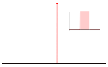
English: Quantum tunneling is another textbook exercise that is better solved in the energy domain. But doing so means that its dynamics stays hidden in the equations. Black: probability density to find a particle at position x. Red: the energy barrier.
The pulse has a narrow gaussian energy distribution centered around 0.7 times the height of the barrier. The inset shows a zoom of what happens inside the barrier. Obviously the curves y-axes aren't comparable, and both were scaled to just fit the frame. |
| Date | |
| Source | https://twitter.com/j_bertolotti/status/1078689353638072321 |
| Author | Jacopo Bertolotti |
| Permission (Reusing this file) |
https://twitter.com/j_bertolotti/status/1030470604418428929 |
Mathematica 11.0 code[edit]
f[e_, V_, a_, b_, x_] :=
 E^((Sqrt[2] Sqrt[-e m + m V] x)/\[HBar]) a +
  E^(-((Sqrt[2] Sqrt[-e m + m V]
      x)/\[HBar])) b; (*Solution of the time-independent Schrodinger \
equation for a constant potential V*)

df[e_, V_, a_, b_, x_] :=
 Evaluate@FullSimplify[D[f[e, V, a, b, x], x] ];
coeff = FullSimplify[Solve[{f[e, V0, 1, b, l1] == f[e, V1, c, d, l1],
    df[e, V0, 1, b, l1] == df[e, V1, c, d, l1],
    f[e, V0, a2, 0, l2] == f[e, V1, c, d, l2],
    df[e, V0, a2, 0, l2] == df[e, V1, c, d, l2]}, {b, c, d,
    a2}] ]; (*impose continuity and smoothness to find all the needed \
coefficients*)
xmin = -100;
xmax = 100;
\[HBar] = 1.;
m = 1.;
V0 = 0;
V1 = 1;
l1 = 5;
l2 = 7;
e =.;
g = Piecewise[{{f[e, V0, 1, b, x] /. coeff,
     x <= l1}, {f[e, V1, c, d, x] /. coeff,
     l1 < x < l2}, {f[e, V0, a2, 0, x] /. coeff,
     x >= l2}}]; (*Complete solution as a function of the energy e*)
\[Sigma] = 0.05;
e0 = 0.5; fevo =
 Table[Flatten[
   Table[(E^(-((e - e0)^2/(2 \[Sigma]^2))) g) /. {e -> j}, {x, xmin,
     xmax, 0.201}]], {j, 0., 1., 0.0011}];
evo = Transpose[InverseFourier /@ (Transpose[fevo]) ];
p1 = Table[If[j != 0,
   Show[
    Plot[50*HeavisidePi[(x - 6)/2], {x, xmin, xmax},
     PlotStyle -> {Red}, Filling -> Bottom],
    ListPlot[Abs[evo[[j]] ]^2, PlotRange -> All,
     DataRange -> {xmin, xmax}, Joined -> True,
     PlotStyle -> {Black}],
    PlotRange -> {0, 50}, Axes -> False,
    Epilog -> Inset[
      Show[
       Plot[50*HeavisidePi[(x - 6)/2], {x, xmin, xmax},
        PlotStyle -> {Red}, Filling -> Bottom],
       ListPlot[Abs[evo[[j]] ]^2, DataRange -> {xmin, xmax},
        Joined -> True, PlotStyle -> {Black}, PlotRange -> All]
       , PlotRange -> {{l1 - 2, l2 + 2}, {0, 15}}, Axes -> False,
       Frame -> True, FrameTicks -> None
       ], {60, 35}, Automatic, 60]
    ]
   ], {j, -25, 25}]
ListAnimate[Drop[p1, {26}]]
Licensing[edit]
I, the copyright holder of this work, hereby publish it under the following license:
| This file is made available under the Creative Commons CC0 1.0 Universal Public Domain Dedication. | |
| The person who associated a work with this deed has dedicated the work to the public domain by waiving all of their rights to the work worldwide under copyright law, including all related and neighboring rights, to the extent allowed by law. You can copy, modify, distribute and perform the work, even for commercial purposes, all without asking permission.
|
This file, which was originally posted to
https://twitter.com/j_bertolotti/status/1030470604418428929, was reviewed on 29 December 2018 by reviewer Ronhjones, who confirmed that it was available there under the stated license on that date.
|
File history
Click on a date/time to view the file as it appeared at that time.
| Date/Time | Thumbnail | Dimensions | User | Comment | |
|---|---|---|---|---|---|
| current | 16:57, 28 December 2018 | | 360 × 223 (188 KB) | Berto (talk | contribs) | User created page with UploadWizard |
You cannot overwrite this file.
File usage on Commons
There are no pages that use this file.